A mathematical framework for thermodynamic computing with applications to chemical reaction networks - npj Unconventional Computing

Generally, in a system of n observables, we have unit vectors along a coordinate axis for each observable, . We define an arbitrary unit vector , such that a distance ξ that measures the extent along x is,

This relationship can be exploited to create an adder function. If there is an observable x due to a process ξ that maps x and x to x (ξ: x + x ↦ x), then addition can be carried out in x-space. Specifically, to add two variables y + y, first define,

where for reasons that will become clear below. Then,

The first term on the right-hand side carries out the mapping x + x ↦ x and the second term maps x ↦ y. The extent of the mapping of each process is determined by the mechanical change in the thermodynamic process, Δξ. Importantly, n addition operations can be easily carried out in parallel if each respective observable x is directly, or indirectly through other x, mapped to a terminal observable x,

Computationally, Eqn (15) is a general adder function for any thermodynamic process. A subtraction function,

can easily be constructed using a similar process but instead of measuring the product of the process x, measure the amount of an intermediate variable x needed to obtain a specific value of the product of the process x. x is thus the subtractant,

Multiplication and division processes similarly follow by exponentiating Eqns (15) or (17). For multiplication,

That is, multiplication and division are obtained by using the same processes as addition and subtraction but not working in space. Concrete examples are given next.

Experimentally, the process of mapping one object to another consists of either a deterministic or stochastic physical process ξ that relates the x objects to x, either directly or through other x that may not be observable. In addition to probability densities, equations of state, defined as any function , can likewise be used for computing. If F is the equation of state, then ξ represents a process that changes the state. Consider the equation of state for an ideal gas, PV = ∑xRT for the case of n gas chambers each of volume f and each containing x moles of the gas. Suppose that ξ controls pistons that move all of the gas from the n chambers into a terminal chamber, initially empty, with volume V at constant temperature T. Since all of the gas from each chamber is emptied, . Then again using ,

In this case, since the system is closed, ΔPV = 0 and ΔxRT is simply PV. In short, addition can be carried out by any thermodynamic process because work is additive. Likewise, as we demonstrate below, the thermodynamic odds of one state to another, which is the exponent of the work to move from one state to another, is multiplicative in nature.

Oxidation-reduction phenomena in chemistry, as well as electrical phenomena, are represented by the thermodynamic equation of state ΔG = - zΔE where G is the free energy, z is a charge and ΔE is an electric potential. If z is a charge transferred due to chemistry (or a charge translocated in an electrical circuit), ξ is the extent of chemical reaction i (or analogously a unit length of the circuit component i), then, again representing , the relevant equations are,

where in Eqn (23) was used. Eqns (22) and (23) describe the additivity of sequential chemical reactions i and voltages of sequential components in a circuit. The carrying out of arithmetic operations using voltages in electrical analog computing, an adder, is well known.

In general for chemical reactions, the chemical free energy is G = ∑xμ where x is the count or concentration of species i and μ is the chemical potential. Then from Eqns (7),

Eqn (25) is the basis for a chemical differential analyzer. For example, the differential equation,

The first integral is simply the work done by the chemical system and the second is proportional to the extent to which the system has reacted (for example, the number of reactants consumed). Consequently,

For a mechanical differential analyzer, the integral is output onto a graph in which the position of the pen is the memory to which are added differentials of the integral. Multiplication can be carried out as the subsequent exponentiation of the integral. However, this need not be the case in thermodynamic computing, as the exponential of the free energy or entropy is the thermodynamic odds of the final state relative to the initial state. Consequently, the value of the exponential can be calculated directly by an appropriate odds ratio involving the ratio of reactant and product concentrations.

To demonstrate multiplication in chemistry using information, consider the reaction,

where the probability of each species i depends on its standard free energy of formation, ,

The normalization factor is Thus, the f is the derivative of the probability density such that,

where the term in brackets is the normalized chemical potential, βμ.

The mapping needed for computing operations is implemented by a chemical reaction ξ where,

in which case is the stoichiometric coefficient.

To compute a multiplication operation such as y ⋅ y = y in chemical space when the number of particles of each species is large, we represent the initial values of the variable y = f with chemical A, y = f with chemical B, and y = f with chemical C where each is given respectively by,

To determine the value of y after the continuous chemical operation ξ, the integral transform that is needed is the one involving the mapping ξ: x + a ↦ x,

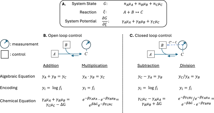
The basic chemical operations corresponding to addition, subtraction, multiplication and division are shown in Fig. 1. In the chemical processes of addition and multiplication, the chemical reactants represent the operands and the chemical product represents the solution. These systems are open-loop control systems: the reactants are controlled and the chemical products are measured. For subtraction and division, at least one product is an operand and at least one reactant is a solution. Subtraction and division are carried out by closed-loop control: a reactant is titrated to obtain the desired chemical product.

To demonstrate the mechanics of the procedure, consider the case in which and f is unknown. Let the standard chemical potentials be given by , , and let the system be at a non-equilibrium steady state in which the counts of the reactants are x = 2, x = 4. is measured. Consequently, the thermodynamic odds of the reaction KQ are known. More precisely,

where the latter term accounts for the change in the probability as the total number of particles changes.

For the purpose of demonstration, the concentration of the product that is to be measured experimentally will simply be determined analytically from chemical thermodynamics (Eqs. (42) and (43)); that is, when KQ = 8. Then carrying out the multiplication in chemistry,

A more insightful and realistic case is to carry out the operation when y and y are both large numbers and using parameters , and from real chemical species. So that we know the exact solution to the problem, we take y and y to be such that,

Choosing a = 1.0 × 10 gives,

First, we choose two convenient chemical species A and B to represent y and y such that y = f, y = f from Eqn (39). For convenience, we will use dihydroxyacetone and glyceraldehyde for A and B, respectively, and fructose for C. Their respective reference chemical potentials at pH = 7.0 and ionic strength 0.25 M are kJ/mol, kJ/mol, and kJ/mol. At T = 298.15, the ambient energy is RT = 2.478956 kJ/mol. The respective counts of the chemicals are,

Assuming that the chemicals are in one liter (1 L) of water, division by Avogadro's number gives concentrations in moles/liter (M),

where N = 6.022141 × 10 mol. Starting with no C present, only a small amount of A and B are allowed to react such that the final concentration of C is measured to be a little less than millimolar, molar. At this concentration, the thermodynamic odds of the reaction are KQ = 1.0 × 10. Then the chemically computed value of y ⋅ y is,

The in-silico chemical calculation compares with the analytical value y ⋅ y = a such that

In this case, the error is due to the limited precision of the computer used to carry out the chemical calculations in-silico. In an actual chemical computer, the error will depend on the measurement precision of the starting material, n and n, the product, n, and on the uncertainty in each of and . However, if calorimetry is used, only the chemical potential of the final product is needed, in that the value of K is the heat released during the reaction. In addition, the precision of the measurements can always be increased in practice through multiple dilutions or concentrations.

In the examples above, the problem of finding the solution of y ⋅ y has been changed to the problem of finding the solution to KQ ⋅ f, and we had to additionally calculate the transforms from f → n, f → n and . Thus, there may or may not be an advantage to using the chemical reactions to solve the multiplication problem in these simple cases.

However, consider a higher-dimensional example, in which we want to find the product f of N + 1 random variables y for i ∈ [0, ..., N],

The chemical process for calculating f is shown in Fig. 2. The chemical system has components {x, ..., x} which are subset into N + 1 reactants r and N products p. The y = f to be multiplied are represented by the chemical reactants r. The p are the reaction products with p being the final product.

The solution f can be determined from the corresponding known reactant concentrations , calculating or measuring K, and measuring p,

The values of the intermediate products p do not have to be stored in memory or even known. K in Eqn (70) is , where 1 is the ones vector and , the vector of known standard chemical potentials, and S is the stoichiometric coefficients for each of the M chemical species (reactants and products) for each of the Z reactions are captured in the stoichiometric matrix,

To add two products together,

the two products are computed independently as described above, such that y = ∏y of N + 1 random variables y and z = ∏z of N + 1 random variables z, as shown in Fig. 3. The value y and z are then the input concentrations for chemicals A and A. The sum of the products is then computed using the chemical reaction A + A = A. The chemical formulation is,

Here r and are the respective reactants involved in the y-product reaction and the z-product reaction. K is , where again 1 is the ones vector and . S is the stoichiometric coefficients for each of the M chemical species (reactants and products) for each of the Z reactions that synthesize y from the reactants r. In Fig. 3, Z = N. Analogous parameters are likewise defined regarding z.

If instead the concentrations of intermediates are measured, then the reaction free energies ΔG for each of the Z reactions can be determined. This allows for matrix-vector multiplication,

in which A is represented by S, the stoichiometric matrix, and in this case f is represented by the vector of chemical potentials, f = μ. The product b is,

This analysis is similar to that found by Aifer, et al., but rather than harmonic potentials, chemical potentials are used. Notably, however, the system is easily generalized beyond equilibrium solutions since non-equilibrium boundary conditions can easily be applied. In this case, the computational solution is found at a non-equilibrium steady state. In principle, non-equilibrium boundary conditions would represent the computational problem through constraints in concentrations included in the probability density (Eqn (21)).

Moreover, given a set of V independent chemical systems k, each with its own stoichiometric matrix S and respective set of mapping processes (reactions) {ξ}, composite computations can be carried out such that,

To bridge the theoretical foundations of CRNs with practical implementations, we build on existing features and suggest the concept of a microfluidic device system designed to execute fundamental chemical computations described above. The system must support digital control interfaces to manipulate and measure signals, chemical compartmentalization strategies to enable execution of multiple operations, feedback mechanisms to chain chemical reactions in time, and consequently computations, and a mechanism to execute complex operations such as f(x) = log(e) enabled by the dynamics of certain species and permeable membranes. We believe prototype systems can be implemented using current microfluidic fabrication techniques, leveraging a wide range of microfluidic technologies discussed below.

Microfluidic technologies have evolved into versatile platforms supporting biological analysis, chemical synthesis, and computational modeling. Early advances focused on cell-based and droplet microfluidics, enabling single-cell manipulation and controlled droplet generation. These systems demonstrated high precision in reagent handling and isolation, establishing foundational mechanisms for reaction control at the microscale. Further developments expanded into biomedical and environmental applications, leveraging new materials and fabrication methods to integrate sensors and achieve biocompatibility and scalability.

Recent research emphasizes programmability, modularity, and adaptive control in microfluidic systems. Digital microfluidics and circuit-based network models introduced flexible droplet actuation schemes, while compiler-assisted and machine-learning-driven control frameworks have automated design and operation. Collectively, these innovations inform the proposed chemical computing architecture, combining precise micro-scale actuation, dynamic feedback control, and programmable digital interfaces to realize computationally capable biochemical systems.

To carry out the needed operations, we propose the system presented in Fig. 4, consisting of a multilayer microfluidic chip that leverages the ideas above, incorporating:

The device operates in three phases:

A programmable controller synchronizes reactant injection, chamber mixing, and measurement. This enables composability of CRN operations in a manner analogous to instruction sequencing in electronic processors.

The microfluidic chip incorporates elastomeric valves, micropumps, and membranes with tunable permeability. These features allow selective coupling of chemical reservoirs, ensuring robust control over concentration dynamics.

Reaction free energies (G) and chemical potentials (μ) act as computational primitives. Open-loop systems leverage direct measurement of product potentials, while closed-loop control dynamically adjusts inflows to converge on the desired result. The membrane-mediated logarithmic transformation provides a mechanism to extend computation to nonlinear functions required for solving ODEs and higher-level mathematical tasks.

By combining precise microfluidic control with thermodynamic principles, the device acts as a biochemical analog computer. Its modularity allows chaining of operations, thereby realizing scalable reservoir computing frameworks. This approach enables experimental validation of CRN-based computation while providing a pathway toward energy-efficient, non-silicon analog computing architectures.