Applying a fractional derivative transforms these inputs into signals that approximate white noise, thereby maximizing entropy and improving the efficiency of spike coding. This implies that fractional-order dynamics are not only biologically plausible but may confer functional advantages by aligning neural dynamics with the statistics of natural sensory inputs.

The introduction of fractional-order dynamics into RC provides control over a fundamental trade-off in how the reservoir processes temporal information. By replacing the standard Leaky Integrate-and-Fire (LIF) with an Fractional-order Leaky Integrate-and-Fire (FLIF), α may be used to control a balance between retaining a rich history of past inputs versus maintaining sensitivity to new environmental signals.

Fractional calculus generalizes the concepts of differentiation and integration to non-integer orders. The most classical definition is the Riemann-Liouville form, which expresses a fractional derivative as an integral operator with a power-law kernel. For a function x(t), the Riemann-Liouville derivative of order α (0 < α < 1) is defined as

where Γ(⋅) is the Gamma function. This formulation makes explicit the non-local nature of fractional differentiation: the present state depends on the entire history of the system, weighted by a power law. Unlike integer-order derivatives, which depend only on instantaneous changes, the Riemann-Liouville derivative encodes memory of all past dynamics.

Two alternative formulations are commonly used in applications. The Grünwald-Letnikov (GL) derivative is defined in terms of finite differences:

where are generalized binomial coefficients. The GL form is particularly useful for numerical simulations, as it lends itself to discrete-time implementations. Accordingly, the GL form is utilized throughout this work.

The Caputo derivative modifies the Riemann-Liouville form by moving differentiation inside the integral:

where denotes the first derivative of x(τ). This definition is often favored in physical modeling because it allows for initial conditions specified in terms of integer-order derivatives, making it compatible with experimentally accessible quantities such as voltages and currents at t = 0.

In practice, the GL and Caputo forms yield very similar dynamical behavior, and both converge to the Riemann-Liouville derivative in the appropriate limits. All three definitions emphasize the same fundamental property: fractional differentiation couples the present dynamics of a system to its entire history, with memory decaying according to a power law.

To connect fractional calculus with RC, the standard LIF neuron is extended to a FLIF neuron model.

The classical LIF neuron describes the membrane potential V(t) as a first-order differential equation with a leak toward the resting potential and input-driven currents. In extending this model to the FLIF model, the first-order derivative is replaced by a fractional derivative of order α, yielding dynamics with long-tailed memory.

A common biophysical form is written in terms of the effective capacitance C and resistance R:

where V is the resting potential and I(t) is the input current.

An equivalent form, which we use throughout this work and in our simulations, rewrites the leak term in terms of the membrane time constant τ = RC:

where b is an optional bias current. This representation is more convenient for numerical implementations, since τ is typically treated as a tunable parameter.

When V(t) reaches a threshold V, the neuron emits a spike and the potential is reset to V.

The introduction of the fractional derivative fundamentally changes the dynamics. For α = 1, the model reduces to the classical LIF neuron with exponential decay. For α < 1, the neuron exhibits a power-law memory kernel, integrating its input with a heavy-tailed weighting of past activity. This produces dynamics consistent with experimental observations of spike-rate adaptation, anomalous diffusion of ions, and the whitening of power-law input signals.

The parameter α thus controls the balance between sensitivity to recent inputs and the retention of long-term history, offering a tunable mechanism for matching neural dynamics to the statistics of input stimuli.

The FLIF neuron provides a compact and biologically grounded way to introduce scale-free memory into artificial neural reservoirs. It also serves as a bridge between theoretical models of fractional dynamics and practical implementations in both software and hardware, making it a natural building block for FOR computing.

In the sections that follow, we adopt the τ-based form in Eq. (5), as it directly corresponds to our software implementation using the Grünwald-Letnikov discretization.

An important consequence of fractional dynamics is a shift in the effective rheobase of the neuron. For α < 1, the fractional derivative acts as an additional dampening term on the membrane potential, reducing the rate at which inputs accumulate toward threshold. This means that lower values of α require stronger input to elicit a spike, effectively raising the rheobase.

Accordingly, to compare across different α values, one must account for this difference in excitability, either by adjusting bias currents or scaling input gain. Without such normalization, reservoirs at lower α may appear artificially quiescent as they are under-driven relative to higher-α systems.

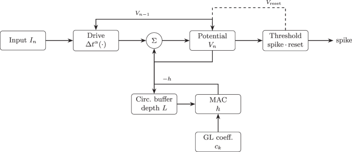
Algorithm 1 summarizes the complete discrete-time update procedure for a single FLIF neuron using the GL discretization; Fig. 1 shows the corresponding signal-flow block diagram.

Algorithm 1

GL-FLIF neuron update

Require: α, Δt, L, τ, b, V, V, V

1: Precompute for k = 1, ..., L

2: Initialize circular buffer , V ← V

3: for each timestep n do

4: Read input current I

5: ⊳ GL history term

7: if V≥V then

8: Emit spike; V ← V

9: end if

10: Push V into circular buffer

11: end for

Information-theoretic analysis

This section establishes the information-theoretic foundation for understanding FORs. We show that the fractional order α acts as a control parameter that simultaneously governs three key computational properties: memory capacity (the ability to store past inputs), AIS (predictability of future states from present states), and information transfer (sensitivity to external inputs). Critically, these properties do not all peak at the same value of α, implying that different tasks will demand different optimal settings depending on their computational requirements.

We begin by formalizing the FOR as an extension of the standard reservoir computing framework, then systematically characterize how α shapes the reservoir's information processing capabilities. This analysis provides the theoretical foundation for understanding why FORs outperform integer-order baselines on certain tasks, and offers principled guidance for selecting α based on task structure.

Formally, a reservoir can be described as a collection of N neurons, each with its own state x(t) and update rule. A general form is

where is the input, W and are the input and recurrent weight matrices, and f(⋅) denotes the neuron model (e.g., standard LIF, fractional LIF). The readout is trained as a linear combination of reservoir states,

with W learned, for example, by regression or another learning rule. In this work, the nonlinear update rules f are implemented as fractional-order neuron models, introducing the order α as a tunable dynamical parameter.

Replacing standard integer-order neurons with fractional-order neurons introduces power-law memory kernels into the reservoir dynamics. The fractional-order α acts as a control parameter, continuously tuning the balance between responsiveness to new inputs and retention of long-term history. To understand the role of α, we analyze the reservoir's information-theoretic and dynamical properties.

A standard measure of reservoir performance is the Memory Capacity (MC), which quantifies how well past inputs can be reconstructed from the present reservoir state. Two forms are relevant here. The linear memory capacity measures the recovery of delayed inputs themselves. For a scalar input sequence {u}, the linear MC at lag k is defined as

where is the optimal linear reconstruction of u from the reservoir state X.

The nonlinear memory capacity extends this definition by replacing u with a nonlinear function of the delayed input. A common choice is to use Legendre polynomials P(u), yielding

The total nonlinear memory capacity is the sum of across lags k and polynomial orders m.

The cumulative memory capacity reported here is the sum of both linear and nonlinear contributions:

This combined measure captures both the ability of the reservoir to store direct input histories and its ability to encode nonlinear transformations of them.

As shown in Fig. 2, empirically, the total (i.e., cumulative) memory capacity decreases with increasing α in an approximately sigmoidal fashion: for low α, the reservoir integrates over long histories and achieves high memory capacity; as α increases, memory decays more rapidly, and at α ≈ 1 the reservoir retains only short-term input traces. This decreasing sigmoid relationship highlights a smooth but sharp transition from history-rich to history-poor dynamics. Interestingly, correlations between neuron activities peak in the transition region of this curve, suggesting that reservoir units are maximally coupled when the system is shifting between long-memory and short-memory regimes. This correlation peak may reflect the presence of critical-like dynamics where the reservoir is most sensitive to both its own state and its external input.

The AIS quantifies how much information the reservoir's present state holds about its immediate future. Formally,

where is the reservoir state vector. For small α, the reservoir's long memory produces an inertial, slow-moving state dominated by the past reservoir states. New inputs act as strong perturbations, and X is therefore not highly predictable from X alone, yielding low AIS.

As α increases, the reservoir becomes more predictably responsive to inputs as the dynamics become dominated by the recurrent structure, thus AIS rises. In other words, higher α values produce reservoirs with more deterministic internal evolution.

The complementary quantity is information transfer, which measures how much of the reservoir's current state reflects the history of the external input. Formally,

where U denotes a delay-embedded representation of the input's past. For low α, the reservoir excels at integrating the input signal, storing substantial information about its external environment. For high α, the reservoir becomes dominated by the dynamics of the recurrent structure of the reservoir, and information transfer from the input decreases.

With reference to Fig. 3, together these measures reveal a fundamental trade-off. Low α values configure the reservoir as a sensitive sensor: highly responsive to external inputs, capable of storing long histories, but internally less predictable. High α values configure the reservoir as a stable internal model: self-determined, predictable, but less permeable to input. At intermediate α, both information transfer and AIS are significant, producing a balance where the reservoir both listens to the input and stabilizes its own dynamics. This intermediate regime, which coincides with the transition in memory capacity and the peak in neuron-to-neuron correlations, represents the most computationally powerful setting.

FORs therefore generalize the standard framework by introducing a tunable continuum of memory and dynamical regimes. The fractional-order α interpolates between input-driven and self-driven dynamics, between long-memory storage and short-memory responsiveness. The balance achieved at intermediate α suggests a critical-like operating point where reservoirs are maximally expressive: capable of capturing external structure, internally stable, and richly interactive. This positions fractional reservoirs as a principled extension of reservoir computing, with information-theoretic properties that can be tuned continuously through α.

Fractional-order neuron implementations

The realization of fractional-order neurons requires translating continuous-time dynamics into discrete or physical forms while preserving the long-memory and power-law characteristics that define fractional systems. Because fractional differentiation is inherently non-local in time, each implementation involves trade-offs among accuracy, computational efficiency, and resource usage. We organize implementations into two primary domains: software-based numerical realizations and hardware-based digital or analog realizations.

In software, fractional dynamics are typically approximated by discrete convolution over past membrane potentials, capturing history-dependent effects through weighted sums with power-law coefficients. This approach allows precise control of parameters such as fractional order α, timestep Δt, and history length L, making it suitable for systematic experimentation and benchmarking. The Grünwald-Letnikov (GL) formulation is particularly advantageous due to its direct correspondence with the continuous fractional derivative and its straightforward implementation as a running sum over stored voltages.

In hardware, fractional-order dynamics can be approximated through digital fixed-point implementations or realized physically through analog elements with inherent fractional characteristics, such as memcapacitive and memristive devices. Digital realizations, particularly those targeting field-programmable gate array (FPGA) or application-specific integrated circuit (ASIC) platforms, enable parallel execution and exploration of scaling behaviors, while analog approaches offer the possibility of directly computing with the physics of fractional-order components. Together, these implementations establish the foundation for practical fractional-order neuromorphic systems, spanning from precise numerical simulation to physical embodiment of fractional dynamics.

Fractional-order software implementations

Simulating fractional-order neurons requires discretizing the continuous-time dynamics. Here we describe the Grünwald-Letnikov (GL) formulation and its direct update rule. For comparison, we briefly note the role of Euler methods commonly used for integer-order LIF models.

The GL form expresses the fractional derivative as a weighted sum over past values:

with timestep Δt, history window length L, and coefficients

Substituting this into the fractional LIF equation with explicit evaluation of the leak term at V yields the practical update rule:

When V≥V, the neuron emits a spike and is reset to V. This direct update aligns with our implementation: a circular buffer maintains past voltages, GL coefficients are precomputed, and the scaling factor Δt ensures consistency across timesteps.

For integer-order LIF neurons (α = 1), the forward Euler method gives the familiar update

while the implicit Euler scheme evaluates the leak at V instead of V, improving stability for stiff systems. The fractional GL update in Eq. (15) can be viewed as a natural generalization: the instantaneous update is still explicit, but past states enter through the convolutional history term with power-law weights.

The principal computational cost of the GL method arises from the history term in Eq. (15). At each timestep, evaluating the convolution requires O(L) operations, where L is the history window length. For long simulations or large networks, this scaling can dominate runtime. The memory requirement is also O(L) per neuron, since each must maintain a buffer of its past voltages.

In practice, L is chosen to balance accuracy and efficiency. Smaller L truncates the power-law kernel, reducing memory effects but lowering cost. Larger L captures the full long-tail dynamics more accurately at the expense of higher runtime and memory. For a reservoir of N neurons simulated over T timesteps, the total cost of the GL convolution is O(N⋅L⋅T), and the memory requirement is O(N⋅L) for the history buffers plus O(L) for the shared coefficient array. For typical values of L used in our benchmarks, this cost is tractable on modern CPUs and GPUs, but becomes a bottleneck when scaling to millions of neurons.

To characterize the accuracy-efficiency trade-off empirically, we swept L from 5 to 250 at α = 0.5 on the FSDD spoken-digit task across 10 trials. Results are shown in Fig. 4.

Accuracy follows a sigmoid-like curve with L: performance is essentially degenerate below L = 30, rises steeply through L ∈ [50, 100], and saturates empirically beyond L ≈ 150. The saturation point is task-dependent, determined by the temporal scale of the relevant history in the input signal; tasks with longer-range dependencies would be expected to saturate at larger L. In the case of FSDD there is a hard upper bound at L = 250, imposed by the sample duration: each sample spans 250 micro-steps (25 macro-steps × Δt = 0.1), so L > 250 cannot add further within-sample history. One practical design choice for FSDD is L = 100, which achieves 93.3% accuracy at the knee of the saturation curve, as beyond L = 100 gains of less than 1% come at linearly increasing compute cost.

Several optimizations exist to mitigate this cost, such as using recursive coefficient updates, Fast Fourier Transforms for long convolutions, or rational transfer-function (IIR) approximations to the power-law kernel. We adopt the direct truncated GL form in this work for clarity and reproducibility.

In hardware realizations of fractional-order neurons, the fractional order α is set by physical device parameters that are subject to manufacturing variation, temperature sensitivity, and long-term drift. We evaluate robustness to two non-ideality scenarios: drift in the realized value of α, and additive noise on the input signal.

We simulated device-level variation in α by training at the nominal α = 0.5 and testing at drifted values ranging from -10% to +10%. As shown in Fig. 5, classification accuracy on the FSDD task is nearly invariant to drift across this range, changing by less than 2 percentage points at ±10% and approximately 0.5 percentage points at ±5%. The near-symmetric response about α = 0.5 is consistent with operation near a local optimum of the accuracy-α curve.

We evaluated robustness to additive i.i.d. Gaussian noise on the input features (σ = 0 to 0.5), simulating sensor noise or signal corruption. Figure 6 compares the fractional reservoir (α = 0.5) against the integer-order baseline (α = 1.0). Performance at α = 0.5 remains stable up to σ = 0.01 and degrades gracefully beyond, while maintaining a consistent accuracy advantage over the integer-order baseline across all tested noise levels.

Notably, the integer-order reservoir shows comparatively less sensitivity to increasing noise, with the performance gap between α = 0.5 and α = 1.0 narrowing at higher σ. Two effects likely contribute to this. The standard LIF acts as a low-pass filter over its membrane time constant, attenuating high-frequency noise components before they influence spiking. In contrast, the fractional LIF incorporates input noise into its power-law memory trace, where it persists across timesteps and is recurrently recirculated through the reservoir dynamics.

Fractional-order hardware implementations

Implementation of fractional-order systems directly in hardware has the potential to improve performance over a software-only implementation, given the opportunity for increased parallelism and the speed advantages of dedicated hardware. A digital hardware implementation may serve as a bridge, allowing for the evaluation of fractional dynamics applied across a range of problems while analog components with fractional characteristics are still in development.

We explore existing work below, including review articles on digital fractional-order systems, as well as two articles describing fractional-order neurons targeting an FPGA execution environment. We then offer an examination of relevant design considerations for digital fractional-order neurons, an overview of a fractional LIF neuron implemented in SystemVerilog, and a discussion of implications for achieving fractional dynamics in a digital context. Regarding a general approach to the implementation of fractional-order calculus in digital systems, review articles and ref. contain mathematical grounding through an overview of fractional-order definitions and options for numerical approximations. Clemente-López et al. address fractional-order systems on both FPGAs and embedded hardware, while Ali et al. focus on FPGAs and their unique architectural features. Both perform tradeoff analysis between different numerical approximation methods and discuss topics most relevant to digital systems, such as discretization techniques and usage of floating-point versus fixed-point representations. Clemente-López et al. highlight the Adomian Decomposition Method as well as the Grünwald-Letnikov (GL) method as the two primary approximation methods used in digital implementations. They further note that the GL method is generally preferred due to its simplicity and flexibility. In ref. , Ali et al. additionally describe the usage of the popular Tustin method for discretization.

The above review articles are in general agreement that the GL method for fractional-order approximation is well-suited for digital platforms. In addition, they both cite the choice to use fixed-point as an appropriate design decision for numerical representation.

In ref. , Malik and Mir present a Hindmarsh Rose (HR) neuron with fractional-order update dynamics. Their work spans single neuron behavior as well as the combined behavior resulting from a coupling of two neurons, with the execution of neuron activity on FPGA. The authors include waveforms showing neuronal dynamics and a range of spiking behavior. Details on representation in hardware include FPGA resource utilization and notes describing the use of a 32-bit fixed-point format.

Similarly, Tolba et al. outline an approach for fractional-order update dynamics in an Izhikevich neuron model executing on an FPGA. They also produced waveforms showing the resulting spiking behaviors, as well as block-level hardware diagrams. Though their work includes greater depth regarding details such as bit widths and routing between high-level components, the focus of the article tends towards the comparison between the integer-order and fractional-order implementations, and the information on engineering tradeoffs and their implications for the fractional-order alone is limited.

As discussed above, selection of α (alpha) determines a system's history retention as well as the relative weighting of recent historical values. This is due to the binomial coefficient magnitudes resulting from a particular value of α at a given timestep, as seen in Eq (13). Figure 7 shows the relative coefficient magnitude decay with increasing timestep for different values of α. Lower values of α provide greater history retention, as seen by the minimal decay in coefficient magnitude, while higher values of α decay much more quickly. In each case, the coefficient magnitude of the historical value at timestep 1 is equal to the value of α itself, so that higher values of α more heavily weight values in recent history.

In the context of digital hardware representation, the memory capacity of a system is dependent on the precision afforded to the binomial coefficient values. If the bit width of the binomial coefficients is too small, the memory capacity will shrink to match the time step with the coefficient magnitude matching the smallest value representable, given the number of bits. Table 1 shows the maximum history length, or value of k, across α values in 3 different fixed-point formats: UQ0.8, UQ0.16, and UQ0.32, where each format is unsigned with zero bits representing the integer component, and 8, 16, or 32 bits, respectively, representing the fractional component.

The required fixed-point representation for binomial coefficients should be determined by the chosen α value for a given application, along with the desired history length. Figure 8 shows the maximum history length for a range of α values in fixed-point formats UQ0.8, UQ0.16, and UQ0.32. An unsigned fixed-point format utilizing 64 bits for the fractional component would allow for a history length of nearly 4 billion, e.g., when using α = 0.9. As such, a fixed-point format of UQ0.64 is likely larger than necessary for most applications, and has the potential to produce time- and space-complexity issues in execution. Conversely, UQ0.16 becomes insufficient at higher α values where rapid coefficient decay limits history to fewer than 100 steps; UQ0.32 is the practical minimum for applications requiring both high α and extended history.

We chose to implement a FLIF neuron using the hardware description language SystemVerilog (SV). Simulation was performed using cocotb, a Python framework targeting chip verification, along with tools from the oss-cad-suite toolchain, such as verilator and gtkwave. Our goal in simulation was to verify the spike timing adaptation described in ref. . We created a preliminary proof-of-concept implementation using a coefficient bit width of 8 and a history length of 8. We iteratively doubled the history length in simulation until the target behaviors were achieved, with a history length of 256 and a coefficient bit width of 16. The final implementation uses Q8.0 fixed-point for input current and membrane potential, and Q0.16 for the GL coefficients. Figure 9 shows the hardware datapath of the implementation, and Fig. 10 summarizes the development pipeline.

We verified that our implementation produced an increasing spike frequency in the presence of a constant input current, as well as a higher recovery spike frequency after a dropout of a constant input current. These findings are consistent with the behavior described by Teka et al. in ref. . Figure 11 shows the increasing spike frequency over time due to the fractional-order system memory. Similar memory effects are seen in Fig. 12, which shows a higher recovery spike frequency than the initial frequency after a brief period of zero input current.

Primary implications of our findings when considering the execution of our design on an FPGA include the identification of available board resources. In particular, the mathematical operations associated with the multiplication and accumulation of coefficients and history terms are ideally mapped to efficient resources such as DSP slices. As the history length grows, the need for DSP slices increases linearly. Similarly, pre-computed binomial coefficient values require storage proportionate to history length.

Intrinsically fractional-order hardware

Analog realizations of fractional dynamics exploit physical devices whose impedance exhibits constant-phase ("fractance") behavior. A promising approach is the fractional-order memcapacitor, whose state-dependent capacitance produces a power-law memory kernel at the circuit level. Recent work has shown that such memcapacitive elements can reproduce neuronal behaviors, including spike-rate adaptation, long-lived responses, and signatures consistent with critical dynamics, positioning them as efficient and biologically plausible neuromorphic primitives.

A practical fractional leaky integrate-and-fire (FLIF) neuron can be realized using four functional components: (i) a leak pathway, (ii) a memcapacitive integrator acting as the fractional memory core, (iii) a Schmitt trigger for robust thresholding, and (iv) a reset switch. In this configuration, the membrane node integrates input current through the memcapacitive branch, producing a slow fractional ramp whose rate depends on the fractional order α. The Schmitt trigger converts this ramp into discrete spikes with hysteresis, while a MOSFET or transmission gate provides the reset path, rapidly discharging the memcapacitor after each spike. Fractional memory effectively increases the rheobase current, so bias and gain normalization across α values are often required to maintain consistent firing thresholds. Schmitt trigger trip points should be chosen so the fractional ramp reliably crosses both thresholds under the expected input range, ensuring stable oscillation and noise immunity.

By embedding the memory kernel directly into the physical capacitance rather than into algorithmic state variables, these designs achieve intrinsic fractional behavior with minimal computational overhead and high analog bandwidth.

When physical fractional-order memcapacitors are unavailable, several well-established approximation methods can emulate their behavior over a target frequency band (ω, ω) corresponding to the neuron's operating spectrum.

The Oustaloup method approximates s (0 < γ < 1) by a stable, minimum-phase IIR filter composed of first-order sections:

where poles and zeros are geometrically distributed between ω and ω, and N controls the approximation order. Larger N broadens the constant-phase region but increases circuit complexity and power consumption; shallow approximations suffice for narrowband operation. ORA maps directly to active-RC or Gm-C biquad sections, and can be implemented in switched-capacitor or mixed-signal IIR topologies.

A finite Foster or Cauer ladder of resistors and capacitors -- referred to here as an R-C network to distinguish it from the reservoir computing (RC) abbreviation used throughout this paper -- approximates a constant-phase element (CPE) whose impedance scales as Z(s) ∝ s over a target frequency band (ω, ω). The pole-zero structure of the ladder, with poles and zeros interlaced along the negative real axis, produces a nearly flat phase response of approximately -πα/2 across the band -- a defining property of a fractional-order element.

This frequency-domain characterization has a direct time-domain counterpart: the impedance Z(s) ∝ s corresponds to convolution with the power-law kernel t/Γ(α), which is precisely the memory kernel underlying the FLIF dynamics described in the Fractional leaky integrate-and-fire neuron subsection. The Grünwald-Letnikov discretization of this kernel (Eq. (13)) approximates the continuous convolution via the weighted sum , where the GL coefficients c decay as k for large k. The R-C ladder thus physically realizes the same power-law memory that the GL algorithm implements in software, providing a direct analog instantiation of the fractional-order neuron's temporal dynamics.

These networks are fully passive, compact, and compatible with SPICE-level modeling. The trade-off between accuracy and area is governed by ladder depth: deeper ladders yield better constant-phase fidelity but at higher component cost.

Together, these methods -- memcapacitive and analog -- demonstrate several design strategies for realizing fractional-order neuronal dynamics.

To illustrate how the theoretical trade-offs identified in the FOR computing subsection manifest in concrete applications, we consider a diverse set of benchmark tasks spanning classification, control, and prediction. These case studies are chosen to highlight complementary aspects of reservoir computation: (i) long-term memory and complex prediction, (ii) efficient representation of natural input signals, (iii) real-time control and stability, and (iv) classification and prediction capabilities.

Specifically, we study:

spoken digit classification,
control of the cart-pole balancing problem, and
classification of blood glucose dynamics for diabetes prediction.

Each task is implemented using a FOR computing framework or a fractional-order spiking neural network (FOSNN), with fractional order α varied systematically.

Together, these examples demonstrate that FORs consistently outperform their integer-order counterparts, and that the benefits align with the theoretical trade-offs in memory, information storage, and sensitivity to natural statistics developed in earlier sections.

Time-series classification

Time-series prediction and classification is a canonical benchmark for reservoir computing, as it simultaneously probes a network's nonlinear transformation capacity and its ability to retain and process temporal dependencies. Here, we evaluate the performance of FORs on the Free Spoken Digit Dataset (FSDD), a widely used corpus for speech-based classification tasks. FSDD consists of short audio recordings of spoken digits (0-9) from multiple speakers, offering natural temporal variability.

The task tests the reservoir's ability to process natural auditory signals that exhibit temporal correlations and spectral regularities common to many real-world sensory signals. As described in the biological motivation discussion above, fractional dynamics may be advantageous in such contexts, as fractional differentiation can act as a flexible signal whitening filter for 1/f-type power spectra.

As shown in Fig. 13, FORs outperform their integer-order counterparts (α = 1.0) on the FSDD task. A complete sweep of α values shows a characteristic peak of accuracy at intermediate fractional orders (α ≈ 0.3-0.5), consistent with the theoretical prediction that optimal information processing occurs where the trade-off between memory retention and whitening balance is achieved. Lower α values yield strong memory but reduced temporal responsiveness, while higher α values approach the Markovian dynamics of standard reservoirs, losing long-range dependencies.

The results above use offline ridge regression as the readout. To confirm that the effectiveness of α is not specific to this choice, we repeated the full sweep using Recursive Least Squares (RLS), an online readout that updates readout weights incrementally as each sample is processed and leaves the reservoir weights unchanged. Figure 14 shows classification accuracy for both methods across α = 0.1-1.0. The two readouts track closely throughout, both peaking at α = 0.5, and the fractional-order advantage over the integer-order baseline is preserved under both. The α optimum and the qualitative shape of the accuracy curve are thus readout-independent, confirming that α controls an intrinsic property of the reservoir dynamics rather than an artifact of the training procedure.

Cart-pole balancing

In this case study, a FOSNN is investigated to test if fractional memory dynamics improve performance and robustness on the cart-pole control task, compared to a standard SNN and multi-layer perceptron (MLP) across a range of α values.

A comparison of model performance on the CartPole-v1 task is shown in Table 2. The MLP displayed the most significant performance change with the introduction of noise, as shown in Fig. 15. The average solve episode and standard deviation increased by 35.35% and 48.18%, respectively. Additionally, the MLP's completion rate decreased by 17%. The standard SNN offered moderate improvements, achieving a slightly higher stability than the MLP in noisy conditions, but it demonstrated a lower completion rate (7.9% loss) and overall performance in comparison to the FOSNN. In contrast, the mid-α FOSNN (α = 0.5-0.7) models displayed similar combinations of higher resilience and absolute performance. The baseline and noisy performances of an α = 0.6 FOSNN is shown in Fig. 16. In general, the mid-α FOSNN group maintained the highest completion rate (98%) while completing the environment the fastest on average (1411 episodes, noisy). Notably, FOSNN (α = 0.7) was the only value to show an absolute improvement in its completion rate (from 95% to 98%), and FOSNN (α = 0.6) improved its standard deviation by 4.32% (from 102.40 to 97.98).

When tested under progressive node removal, the MLP showed the greatest overall robustness, achieving a normalized area under curve (AUC) of 0.540, a lower standard deviation of 43.47, and a critical damage threshold (CDT) of 70%. In comparison, while most FOSNN models were less robust than the MLP architecture, the FOSNN (α = 0.8) showed one notable advantage with the lowest magnitude of initial performance loss, with an initial degradation rate (IDR) of -4.04, as shown in Fig. 17.

Diabetes prediction

The diabetes prediction task evaluates the reservoir's ability to identify diagnostic patterns from physiological time-series data.

Figure 18 shows the effect of varying the fractional order α on performance. Both accuracy and F1 score decreased monotonically as α increased, revealing that reservoirs with stronger memory effects (lower α) achieve superior predictive accuracy on physiological time-series data. The best performance was achieved near α = 0.1, corresponding to a long memory kernel and slower voltage decay, which effectively integrates temporal correlations across patient features. At higher α values, the network dynamics approach the Markovian regime of standard LIF neurons, leading to diminished temporal representation and reduced discriminative power.

A comparative evaluation of all four network architectures is shown in Fig. 19 and Table 3. The FOR achieved the highest mean accuracy and F1 score, outperforming both the standard reservoir and feedforward models. While the MLP and SNN exhibited similar performance, the inclusion of recurrent dynamics in both reservoir variants yielded substantial gains, confirming that temporal integration -- especially when extended by fractional memory -- plays a key role in representing slow-varying physiological processes.

Fractional-order systems for neuromorphic computing: software and hardware opportunities and challenges - npj Unconventional Computing